
 Full Text (PDF)
Abstract
Accurate estimation of discharge in rivers forms the basis of efficient flood management and surface water planning. However, continuous measurement of discharge in a stream is impractical, therefore, discharge in natural streams is generally estimated using the stage-discharge relationship. The reliability of discharge predicted from rating curve depends on the accuracy of the method used in developing stage-discharge relationship. Generalized Reduced Gradient (GRG) solver has been reported as a powerful optimization tool for handling nonlinear optimization problems, therefore, present work is an implementation of Generalized Reduced Gradient technique to determine rating curve parameters. Spreadsheet based non-linear optimization has been applied to model the rating curve for two gauging sites viz. Walton site on Choctawhatchee river and Philadelphia site on Schuylkill river, USA. The stage-discharge relationships for the two sites were also developed by using Genetic Algorithm (GA) and classical rating curve approach rating curve. Comparison of results shows that rating curve equations developed by using GRG technique are as effective as those developed by GA and more accurate than classical rating curve approach. The goodness of fit criteria for both the sites shows that the rating curves obtained by using GRG technique fit the observed data better than classical rating curve approach.
License
This is an open access article distributed under the Creative Commons Attribution License which permits unrestricted use, distribution, and reproduction in any medium, provided the original work is properly cited.
Article Type: Research Article
AQUADEMIA, Volume 1, Issue 2, 2017, Article No: 05
https://doi.org/10.20897/awet/81286
Publication date: 30 Dec 2017
Article Views: 5777
Article Downloads: 4396
Open Access HTML Content References How to cite this articleHTML Content
INTRODUCTION
Streamflow measurement is the basic data required for most of the hydrologic studies such as flood frequency analysis, flood plain zoning, sediment studies, water demand and computation of standard project flood. Accurate stream flow measurement plays a vital role in accurate determination of peak discharge required for the safe and economic design of various hydraulic structures.
Developing rating curves has remained an area of interest of hydrologists and has been interchangeably studied by hydrologists. Stage discharge relationship was established using graphical method by Herschy (1995). Polynomial models for stage discharge relationships were also proposed by Herschy (1995, 1999). Tawfik et al. (1997) applied multilayer artificial neural network (ANN) for modelling the rating curve. Jain and Chalisgaonkar (2000) used ANN for modelling stage discharge relationship for Kolar river and Jamtara site on river Narmada. They also successfully utilised ANN to model the hypothetical hysteresis loop curve for unsteady flow condition. To assess the performance of radial basis function (RBF) neural network for modelling the rating curves Sudheer and Jain (2003) analysed the data set of Jain and Chalisgaonkar (2000) and reported RBF to be better than back propagation multilayer perceptron model. Deka and Chandramouli (2003) presented the application of fuzzy integrated neural network for developing a reliable stage discharge relationship (Zakwan et al., 2017). Bhattacharya and Solomatine (2005) established stage discharge relationship using model tree M5 and ANN reporting the reliability of model tree M5 and ANN are comparable in estimating the discharge. Sivapragasam and Muttil (2005) proposed the use of Support Vector Machine (SVM) for extrapolating the rating curve. Moyeed and Clarke (2005) used Bayesian methods for fitting rating curves. Stage discharge relationship for coastal low- gradient streams was developed by Habib and Meselhe (2006) using ANN and nonparametric regression. Peterson-Øverleir (2006) introduced a method based on the Jones formula and nonlinear regression to model the stage discharge relationship where the stage discharge relationship is affected by hysteresis resulting from unsteady flow. Compound neural network was employed by Jain (2008) to develop a relationship between stage discharge and suspended sediments. Guven and Aytek (2009) established stage discharge relationship by GEP (Gene Expression programming) for two American rivers. Goel and Pal (2011) employed Support Vector Machine (SVM) to develop stage discharge relationship for two sites on Indian rivers and successfully traced hypothetical looped rating curve by dividing the data into rising and falling stage data. Mir and Dubeau (2014) outlined the limitations of earlier approaches and proposed the use of curvilinear asymptotes rather than straight ones. Wolfs and Willems (2014) developed stage-discharge curves affected by hysteresis using four different approaches that included single rating curve, rating curve with state dependent parameter (dynamic correction), artificial neural network (ANN) and model tree (M5). Considering the case studies of river Marke and river Dender they concluded that state dependent parameter rating curve is most suitable approach for most of the cases and gives better physical interpretation of the problem. Atiaa (2015) modelled rating curve using ANN, Takagi-Suegeno (TS) fuzzy interference and model tree, reporting model tree M5P and TS fuzzy as quite reliable for establishing the rating curves. Londhe and Panse-Aglave (2015) presented comparative analysis of ANN, MT and nonlinear regression method for modelling stage discharge curve. ANN and MT performed equally well for estimation of discharge however, MT appear to be more transparent than ANN. Ghorbani et al. (2016) compared the performance of SVM, ANN, MLR and simple rating curve (RC) reporting SVM to be best among them for estimating the discharge. Maghrebi and Ahmadi (2017) proposed a new approach for modelling discharge rating curve using isovel contours with the corresponding hydro-geometric parameters of the cross sections and dimensional analysis to interrelate the discharges at two different stages, however, such detailed data at sites is rarely available.
Ghimire and Reddy (2010) utilised GA (Genetic algorithm) and Model Tree to establish discharge rating curve, reporting the superiority of GA over GEP and MT in developing the stage discharge relationship. This paper presents the application of spreadsheet based GRG technique to establish the discharge rating curves and compares the performance of GRG with GA.
METHODOLOGY
Rating curve: Continuous measurement of discharge is very costly, time consuming and impractical during floods, therefore, in majority of the streams measurement of discharge is made by indirect means of establishing a relation between stage and discharge. This relationship when expressed graphically is known as rating curve. Discharge through a river section is influenced by channel properties, flow characteristics, bed slope and many other factors, however, quantification of all these factors at every time step is impractical (Zakwan et al., 2017). Rating curve is believed to represent the combined effect of many flow and channel parameters and hence, can be used to estimate the discharge with reasonable accuracy. Historical stage discharge data from gauging station is used to establish the dependency of discharge on stage by plotting the graph between the observed discharge and corresponding stage of river. The stage discharge data to be used for establishing rating curve should include almost all the possible range of stage that can occur at a section as extrapolation of rating curve is not generally allowed. Once the rating curve has been established for a gauging site, discharge can easily be estimated from the observed stages alone. Thereby, eliminating the need of rigorous, repetitive, time consuming, costly and sometime impractical exercise of continuous discharge measurement (Muzzammil et al., 2015). Water surface elevation in a stream can be measured continuously in a relatively inexpensive manner than discharge in stream. The general form of rating curve equation may be represented as
| \[Q\ = \ K{(G - a)}^{n}\] | (1) |
where \(Q\) = Stream discharge; \(G\) = Stage height; \(a\) = A constant representing the gauge reading corresponding to zero discharge; \(K\) and \(n\) are the rating curve constants.
In Equation (1) the constant \(a\) corresponds to the gauge height for zero discharge in stream. Being a hypothetical parameter \(a\) cannot be determined in field and hence generally graphical methods are employed to estimate its value (Subramanya, 2008).
Parameter Estimation: \(K\), \(a\) and \(n\) are the parameters in the rating curve equation. Graphical methods are employed to estimate its value of \(a\). Traditionally best fit value of \(K\) and \(n\) are obtained by regression. The logarithmic form of Equation (1) may be written as
| \[log\ Q\ = \ n\log{(G - a)} + \log K\] | (2) |
which may be expressed as
| \[Y = AX + B\] | (3) |
where \(Y = \log Q\); \(A = n\); \(X = \log{(G - a)}\); \(B = \log K\).
Using regression analysis, the values of \(A\) and \(B\) can be calculated through following relations
| \[A = \frac{N(\sum_{}^{}{XY) - (\sum_{}^{}X)(\sum_{}^{}{Y)}}}{N\left( \sum_{}^{}X^{2} \right) - {(\sum_{}^{}X)}^{2}}\] | (4) | |
| \[B = \frac{\sum_{}^{}{Y - A\ (\sum_{}^{}X)}}{N}\] | (5) |
where \(Y = \log Q\) and \(X = \log{(G - a)}\).
Values of \(n\) and \(K\) can be calculated utilizing the above-mentioned equations. Avoiding such a tedious process, optimization techniques may directly estimate rating curve parameters. One such optimization technique known as Generalized gradient (GRG) technique has been used in the present study to estimate the rating curve parameters.
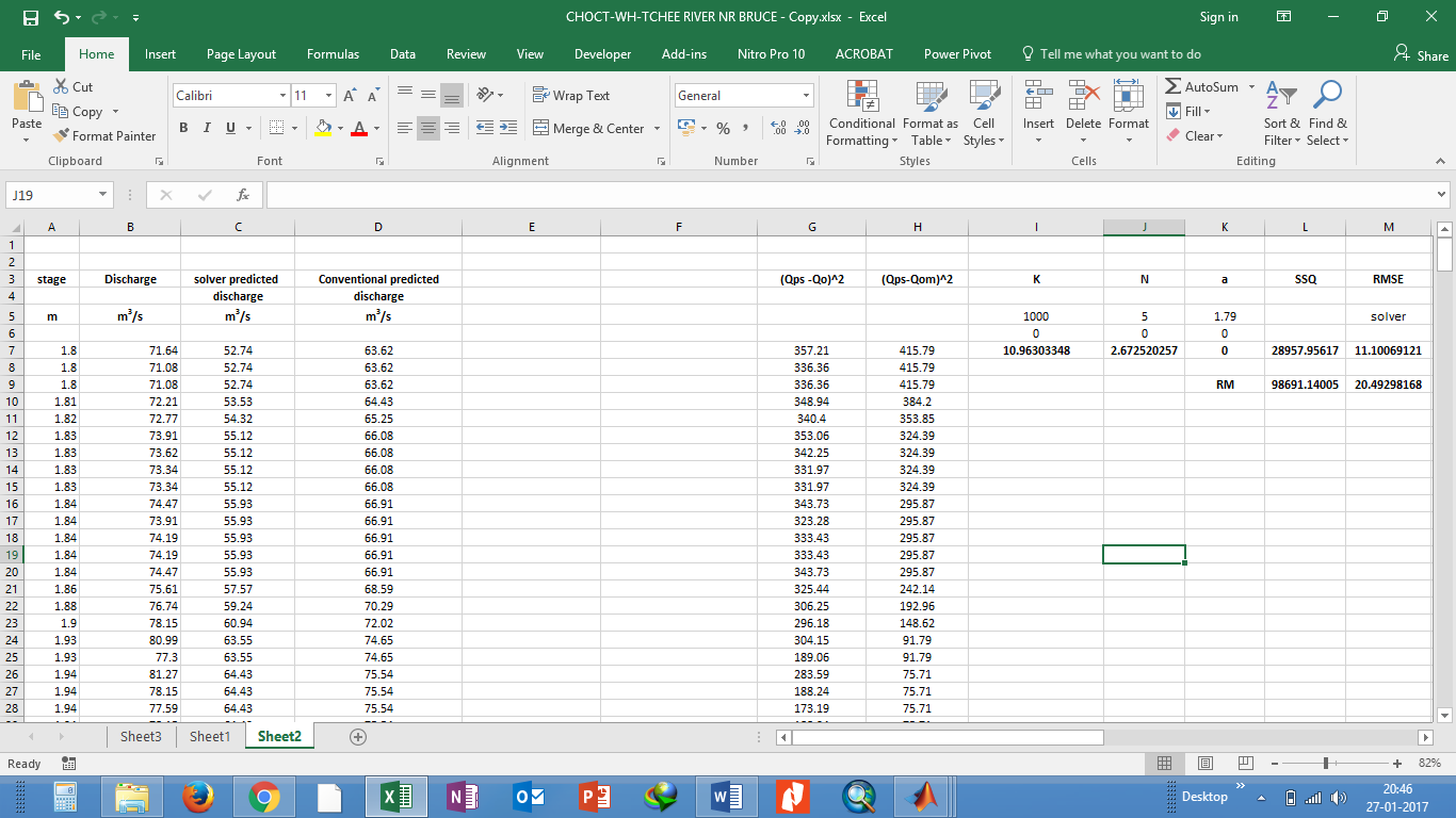
To estimate the rating curve parameters using GRG technique the observed stage discharge data was fed into the spreadsheet sheet. Discharge for each stage was calculated using Equation (1) based on the assumed value of parameters in the variable cells. Using GRG with appropriate bound on rating curve parameters, objective function was optimized to obtain the optimal values of the parameters for the rating curves. Minimization of sum of square of error between observed discharge and predicted discharge was used as an objective function which may be presented as
| \[\text{Min SSQ} = \sum_{i = 1}^{N}\left\lbrack Q_{\text{observed}}^{i} - (K({G - a)}^{n}) \right\rbrack^{2}.\] | (6) |
The numerical set up of the problems for GRG method is shown in Figure 1.
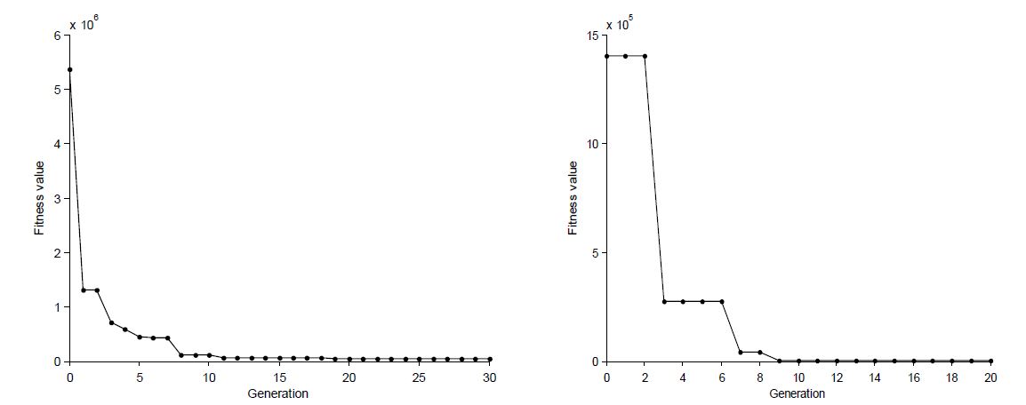
To apply genetic algorithm a program for objective function (Equation (6)) was written in Matlab environment to obtain the optimal rating curve parameters. Graphical User Interface of GA in Matlab was used to assign the various parameters such as population size, generation and tolerance function. In the present study uniform creation function with population size 50 and rank scaling was used. Further, the mutation function and migration were set as adaptive feasible and forward respectively. The number of generation were decided based on the plots of fitness verses generation curves as shown in Figure 2. Sudden decrease in the objective function in Figure 2 may represent successful mutations.
GRG TECHNIQUE
GRG solver is an optimization tool in Microsoft excel which may be used to obtain the optimum values of parameters of linear as well as nonlinear equations. Solver methods in MS excel consist of LP solver (linear programming solver) for linear equations, GRG solver (Generalized Reduced Gradient) and Evolutionary solver for optimization of nonlinear equations.
GRG solver is a nonlinear optimization code developed by Lasdon et al. (1978). GRG and its specific implementations have been proved over many years as one of the most robust and reliable approach to solve difficult nonlinear programming problems (Lasdon and Smith, 1992). Two techniques are used to determine the search direction in GRG solver. The default choice is quasi-Newton method which is gradient based technique and the other choice is the conjugate gradient method. Depending on the available storage GRG solver can switch between quasi-Newton and conjugate gradient method (Zakwan et al. 2016). Evolutionary solver is a hybrid of evolutionary and genetic algorithms and classical optimization methods which includes classical gradient based quasi-Newton methods, gradient-free direct search methods and simplex method. Evolutionary solver is a hybrid of genetic and evolutionary algorithms and classical optimization methods, including gradient-free direct search methods, classical gradient based quasi-Newton methods and even simplex method. GRG solver stops if the absolute value of relative change in the objective function is less than the tolerance value for the last five iterations while the evolutionary solver stops when ninety-nine percent of population members have fitness values within the convergence tolerance of each other. Rating curve equations are nonlinear equations therefore, GRG nonlinear solver was used to obtain the optimum values of the parameters. GRG solver algorithm has been formulated in FORTRAN language consisting of main program and a number of subroutines. The values of decision variables are considered to be optimal if the Kuhn-Tucker optimality conditions are satisfied to within EPSTOP (user defined small positive number having 10-4 as default value) or the fractional changes in the value of objective function is less than EPSTOP for a number of consecutive iterations.
Microsoft excel has been in use over several years in various fields of engineering. Hegazy and Ersahin (2001) optimized overall construction schedule using excel. Low and Tang (2001) used excel solver to assess the reliability of embankments on soft ground. Simplicity and ease to handle solver lured Jewell (2001) to demonstrate the utility of equation solvers in hydraulic design. Bhattacharjya (2010) utilised excel solver to determine critical depths in conduits. Barati (2013) successfully applied excel solver to estimate the parameters of nonlinear Muskingum models for flood routing. On comparison, sum of square of error in outflow estimation for excel solver was minimum among least square method (LSM), Hook-Jeeves and Davidson-Fletcher-Powell (HJ+DFP), Genetic algorithm (GA) and Immune clonal selection algorithm (ICSA). Application of GRG solver have also been found to obtain the parameter of infiltration equations (Zakwan et al., 2016; Zakwan, 2017). Parameters of Intensity Duration Frequency (IDF) were also estimated through application of GRG solver by Zakwan (2016).
GENETIC ALGORITHM
Genetic algorithm is an optimization technique involving natural selection and genetics, formulated on the principles of Darwin’s theory of survival of the fittest. This technique was developed by John Holland (1975) which was finally popularized by Goldberg (1989). The idea in genetic algorithm is to initiate the search with random population of candidate solutions for the actual objective function rather than its derivative, based on operators derived from natural genetic variation and natural selection such as mutation, inheritance, selection, and crossover. Next generation chromosomes (children) are generated from the selected set of chromosomes (parents) based on the value of the fitness function. The better fitted individuals are granted higher chances of reproduction. In case of minimization problems, the set of chromosomes (parents) producing lower objective function are considered as better fit. Crossover allows extraction of best characteristic from both chromosome (parents) to generate better chromosome (children). Mutation takes care of diversity of population and avoids trapping of search into a local optimum. Mutation results in rapid changes in the objective function there by making it possible to explore wider regions (Gutowski, 2005). As GA, does not rely on the derivative of the objective function it can also be used for optimization of discontinuous functions.
DATA
Mean daily stage-discharge data of Choctawhatchee river at Walton (Station no: 02366500, Latitude 30º27'03'' and Longitude 85º53'54'', USA) and Schuylkill River at Philadelphia (Station no: 01474500, Latitude 39º58'04'' and Longitude 75º11'20'', USA) was obtained from USGS website (USGS website, http://www.usgs.gov.) for the period of September 2015 to September 2016. Initial 70% data (255 observation) was used for calibration and remaining 30% data (110 observation) was used for validation of developed relationships for either site i.e. the daily data from September 2015 to April 2016 was used for calibration and the developed equations were validated using rest of the data. Some of the statistical parameters of these data sets are shown in Table 1. Walton station on Choctawhatchee river has a drainage area of about twelve thousand square kilometres. Philadelphia station is about fifty meters upstream of Fairmount Dam and has a drainage area of about 5000 km2.
|
Table 1. Statistical parameters for the Stage-discharge data
|
RESULTS AND DISCUSSION
The rating curve parameters \(a\), \(K\), and \(n\) were estimated using classical rating curve method (RM), nonlinear optimization methods that include GRG and GA. The parameters were estimated by the methodology as described earlier. The parameters estimated by the nonlinear optimization methods were almost the same. However, the time required to obtain the optimal parameters GA was much longer than GRG method. This may be attributed to the fact that for convex analytical function calculus based method outperform genetic and evolutionary based method (Haupt and Haupt, 2004). The values of rating curve parameters based on classical rating curve method (RM), GRG and GA have been reported in Table 2.
|
Table 2. Rating curve parameters for different sites
|
The performance of various methods for the parameter estimation was assessed with respect to the relation between the observed and the estimated discharges based on the following indices
| Root mean square (RMSE) = \(\sqrt{\frac{\sum_{i = 1}^{n}{({Q_{o_{i}} - Q_{e_{i}})}^{2}}}{N}}\) | (7) | |
| Nash-Sutcliffe (1970) criteria (e) = \(\left\lbrack 1 - \frac{\sum_{i = 1}^{N}{(Q_{o_{i}} - Q_{e_{i}})}^{2}}{\sum_{i = 1}^{N}{(Q_{o_{i}} - \overset{\overline{}}{Q})}^{2}} \right\rbrack\) | (8) | |
| Correlation coefficient (r) = \(\frac{N(\sum_{}^{}{Q_{o}Q_{e}}) - (\sum_{}^{}{Q_{e})(\sum_{}^{}{Q_{o})}}}{\sqrt{(N(\sum_{}^{}{({Q_{e}}^{2}}}) - \left( \sum_{}^{}Q_{e} \right)^{2})(N\left( \sum_{}^{}{Q_{o}}^{2} \right) - ({\sum_{}^{}{Q_{o})}}^{2})}\) | (9) |
where \(Q_{o}\) is observed discharge; \(Q_{e}\) is estimated discharge and \(\overset{\overline{}}{Q}\) is mean of observed discharge and \(N\) is the number of observations.
| Mean Absolute Relative Error (MAPE) = \(\frac{1}{N}\sum_{i = 1}^{N}\frac{\left| Q_{o_{i}} - Q_{e_{i}} \right| \times 100}{Q_{o_{i}}}\) | (10) |
where \(Q_{o}\) is observed discharge; \(Q_{e}\) is estimated discharge and \(\overset{\overline{}}{Q}\) is mean of observed discharge.
The estimation method with lowest error and the highest correlation coefficient would be considered as the best method. The values performance indices as calculated for both the data sets during calibration and validation have been provided in Table 3 and Table 4. The values of root mean square error, mean absolute error were observed to be the highest, while the efficiency was lowest for classical regression method (RM) during calibration as well as validation which may be attributed to bias introduced as a result of logarithmic transformation of data set to apply linear regression (Ferguson, 1986; Zakwan, 2017). When GA or GRG is applied no such transformation in data is required there by avoiding a bias in the estimates. The performance indices obtained for GRG and GA were approximately the same resulting from equal values of parameters.
|
Table 3. Performance indices for two sites during calibration
|
||||||||||||||||||||||||||||||||||||||
|
Table 4. Performance indices for two sites during validation
|
Table 3 and Table 4 clearly demonstrate that the performance of nonlinear optimization methods is better than that of the classical rating curve method (RM). The reduction in root mean square error (RMSE) using nonlinear optimization methods such as GRG was about 45% and 27% in comparison to RM for Walton and Philadelphia sites respectively. Further, the goodness of fit criteria (Nash criteria and correlation coefficient) for both the sites shows that the rating curves obtained by using nonlinear optimization method fit the observed data better classical rating curve method.
Present results also show that GRG technique is as efficient in optimizing rating curve parameters as GA for both the sites. Ghimire and Reddy (2010) demonstrated the superiority of GA over GEP (Gene Expression Programming) and MT (Model Tree) in estimating the stage discharge relationship. However, tuning of parameter in GA is a difficult, tedious and time-consuming process. Further, it has been observed that the results of genetic algorithm are highly dependent on the initial values of rating curve parameters. The objective function in case of discharge rating curve is generally convex continuous function and for functions of such nature simple calculus based deterministic optimization tools can prove as a reliable source, on the other hand GA is more suitable for functions involving very high degree of nonlinearity, discontinuity or concavity (Haupt and Haupt, 2004). The parameters used to control the optimization process of genetic algorithm (population size, crossover, number of generations and mutation rate) can greatly influence the quality and efficiency of the final solution. These parameters must be defined before the algorithm is used, however, determining the best set of parameter values can be extremely difficult and highly problem dependent (Kingston et al., 2008). No universal rules have yet been found for determining best parameters in GA. Generally, parameter values are determined based on experience and trial-and-error, which can be time consuming and computationally expensive (Kingston et al., 2008). Therefore, a very simple GRG technique has been proposed in this paper to model the rating curve. many researchers have also proposed the use of ANN for modelling rating curves, however, training complex ANN periodically is a cumbersome task and do not yield the functional form of stage discharge relationship (Aytek and Kisi, 2008). Moreover, ANNs and model trees may involve discharge from previous time step as an input in estimating discharge for current stage which may lead to propagation of errors (Aytek and Kisi, 2008).
CONCLUSION
Rating curves were developed for two sites using linear regression as well as nonlinear optimization methods such as GRG and GA. The stage discharge data was divided into calibration and validation data sets. The performance of these method was assessed using root mean square error, mean absolute percentage error, Nash efficiency and correlation coefficient. Values of these indices obtained during calibration as well as validation clearly establish the superiority of nonlinear optimization methods over the classical rating curve method. However, among the nonlinear optimization methods GRG technique has been found to be a powerful, easy and promising tool to predict parameters of nonlinear equations such as stage discharge relationship. Even in case of non-convex complex functions GRG can overcome the problem of local optimum trapping with the Multistart option. It is so simple that even without the knowledge of complicated programming techniques, exact mathematics of optimization and complex parameter tuning as in case of most of optimization methods such as GA and GRG, it can be used to estimate the parameters of rating curve quite accurately. Unlike many other soft computing techniques, it does not obscure theoretical background of the problem and can be easily used by the hydrologic offices to develop the rating curves periodically. Spreadsheet based GRG technique opens a scope for easy solution of wide variety of problems not only in engineering hydrology but also other fields of engineering.
References
- Atiaa, M. (2015). Modelling of stage-discharge relationship for the Gharraf river, Southern Iraq by using data driven techniques: A case study. Water Util. J., (9), pp. 31-46.
- Aytek, A. and Kisi, O. (2008). A Genetic Programming Approach to Suspended Sediment Modelling. J. Hydrol., 351(3-4), pp. 288-298. https://doi.org/10.1016/j.jhydrol.2007.12.005
- Barati, R. (2013). Application of excel solver for parameter estimation of the nonlinear Muskingum models. KSCE J. of Civ. Eng., 17(5), pp. 1139–1148. https://doi.org/10.1007/s12205-013-0037-2
- Bhattacharya, B. and Solomatine, D.P. (2005). Neural networks and M5 model trees in modelling water level-discharge relationship. J. Neurocomp, 63(2005), pp. 381-396. https://doi.org/10.1016/j.neucom.2004.04.016
- Bhattacharjya, R.K. (2010). Discussion of “Evolutionary algorithm for the determination of critical depths in conduits”. J. Irrig. Drain. Eng., 136(3). https://doi.org/10.1061/(ASCE)IR.1943-4774.0000201
- Deka, P. and Chandramouli, V. (2003). Fuzzy-neural network model for deriving river stage discharge relationship. Hydrol. Sci. J., 48(2), pp. 197-209. https://doi.org/10.1623/hysj.48.2.197.44697
- Ferguson, R.I. (1986). River loads underestimated by rating curves. Water Resour. Res., 22(1), pp. 74-76. https://doi.org/10.1029/WR022i001p00074
- Ghimire, B.N.S. and Reddy, M.J. (2010). Development of stage-discharge rating curve in river using genetic algorithms and model tree. International Workshop on Advances in Statistical Hydrology, Taormina, Italy.
- Ghorbani, M.A., Khatibi, R., Goel, A., FazeliFard, M.H. and Azani, A. (2016). Modelling river discharge time series using support vector machine and artificial neural networks. Environmental Earth Sciences, 75(8), pp. 1-13. https://doi.org/10.1007/s12665-016-5435-6
- Goel, A., and Pal, M. (2011). Stage-discharge modelling using Support Vector Machine. IJE Trans. A, 25(1), pp. 1-9.
- Goldberg, D.E. (1989). Genetic algorithms in search, optimization, and machine learning. Boston:Addison-Wesley.
- Gutowski, M.W. (2005). Biology, physics, small worlds and genetic algorithms. Leading Edge Computer Science Research, ed. Susan Shannon (pp. 165-218). Hauppage, NY: Nova Science Publishers Inc.
- Guven, A. and Aytek, A. (2009). New approach for stage-discharge relationship: Gene Expression Programming. J. of Hydrol. Eng., 14(8), pp. 482-492. https://doi.org/10.1061/(ASCE)HE.1943-5584.0000044
- Habib, E.H. and Meselhe, E.A. (2006). Stage-discharge relations for low-gradient tidal streams using data-driven models. J. of Hydraul. Eng., 132(5), pp. 482-492. https://doi.org/10.1061/(ASCE)0733-9429(2006)132:5(482)
- Haupt, R.L. and Haupt, S.E. (2004). Practical genetic algorithms. Second edition. New Jersey, USA: John Wiley & Sons.
- Hegazy, T. and Ersahin, T. (2001). Simplified spreadsheet solution overall construction optimization. J. of Cons. and Manag. Eng., 127(6), pp. 469-475. https://doi.org/10.1061/(ASCE)0733-9364(2001)127:6(469)
- Herschy, R.W. (1995). Streamflow measurement. Second edition. London: E & FN Spon.
- Herschy, R.W. (1999). Uncertainties in hydrometric measurements. In: Hydrometry: Principles and Practice. Second edition, Chichester, UK: John Wiley & Sons.
- Holland, J.H. (1975). Adaptation in Natural and Artificial Systems. Ann Arbor, MI: Univ. of Mich. Press.
- Jain, S.K. (2008). Development of integrated discharge and sediment rating relation using a compound neural network. J. of Hydrol. Eng., 13(3), pp. 124-131. https://doi.org/10.1061/(ASCE)1084-0699(2008)13:3(124)
- Jain, S.K. and Chalisgaonkar, D. (2000). Setting up stage-discharge relations using ANN. J. Hydrol. Eng., 5(4), pp. 428-433. https://doi.org/10.1061/(ASCE)1084-0699(2000)5:4(428)
- Jewell, T.K. (2001). Teaching hydraulic design using equation solvers. J. Hydraul. Eng., 127(12), pp. 1013-1021. https://doi.org/10.1061/(ASCE)0733-9429(2001)127:12(1013)
- Kingston, G.B., Dandy, G.C. and Maier, H.R. (2008). Review of artificial intelligence techniques and their applications to hydrological modelling and water resources management Part 2–optimization. Water Resources Research Progress, pp. 67-99.
- Lasdon, L.S. and Smith, S. (1992). Solving sparse nonlinear programs using GRG. ORSA J. on Com., 4(1), pp. 2-15. https://doi.org/10.1287/ijoc.4.1.2
- Lasdon, L.S., Waren, A.D., Jain, A. and Ratner, M. (1978). Design and testing of a generalized reduced gradient code for nonlinear programming. ACM Trans. on Mathematical Soft., 4(1), pp. 34-50. https://doi.org/10.1145/355769.355773
- Londhe, S. and Panse-Aglave, G. (2015). Modelling Stage–Discharge Relationship using Data-Driven Techniques. ISH J. Hydraul. Eng., 21(2), pp. 207-215. https://doi.org/10.1080/09715010.2015.1007092
- Low, B.K. and Tang, W.H. (2001). Reliability of embankments on soft grounds using constrained optimization. Proc. Third Inter. Con. on soft soil. Hong Kong, China.
- Maghrebi, M.F. and Ahmadi. A. (2017). Stage-discharge prediction in natural rivers using an innovative approach. J. of Hydrol., 545, pp. 172-181. https://doi.org/10.1016/j.jhydrol.2016.12.026
- Mir, Y. and Dubeau, F. (2014). Least square fitting of the stage-discharge relationship using smooth models with curvilinear asymptotes. Hydrol. Sci. J., 60(10), pp. 1797-1812. https://doi.org/10.1080/02626667.2014.935779
- Moyeed, R.A. and Clarke, R.T. (2005). The use of Bayesian methods for fitting rating curves, with case studies. Adv. W. Resour., 28, pp. 807-981. https://doi.org/10.1016/j.advwatres.2005.02.005
- Muzzammil, M., Alam, J. and Zakwan, M. (2015). An optimization technique for estimation of rating curve parameters. Nation. Symp. Hydrol., pp. 234–240, New Delhi.
- Nash, J.E. and Sutcliffe, J.V. (1970). River flow forecasting through conceptual models part I—A discussion of principles. Journal of hydrology, 10(3), pp. 282-290. https://doi.org/10.1016/0022-1694(70)90255-6
- Petersen-Øverleir, A. (2006). Modelling stage-discharge relationships affected by hysteresis using the Jones formula and nonlinear regression. J. of Hydrol. Sci., 51(3), pp. 365-388. https://doi.org/10.1623/hysj.51.3.365
- Sivapragasam C. and Muttil N., (2005). Discharge rating curve extension – A new Approach. Water Resour. Manage, 19, pp. 505-520. https://doi.org/10.1007/s11269-005-6811-2
- Subramanya, K., (2008). Engineering Hydrology. Third edition. New Delhi: Tata McGraw-Hill.
- Sudheer, K.P. and Jain, S.K. (2003). Radial basis function Neural Network for modelling rating curves. J. of Hydrol. Eng., 8(3), pp. 161-164. https://doi.org/10.1061/(ASCE)1084-0699(2003)8:3(161)
- Tawfik, M., Ibrahim, A. and Fahmy, H. (1997). Hysteresis sensitive Neural Network for modelling rating curves. J. of Com. Civ. Eng., 11(3), pp. 206-211. https://doi.org/10.1061/(ASCE)0887-3801(1997)11:3(206)
- USGS (2017) [online] Available at: http://www.usgs.gov
- Wolfs, V. and Willems, P. (2014). Development of a stage-discharge curve affected by hysteresis using time varying model, model trees and neural networks. Env. Mod. Soft., 55(2014), pp. 107-119. https://doi.org/10.1016/j.envsoft.2014.01.021
- Zakwan, M. (2016). Application of optimization technique to estimate IDF Parameters. Water and Energy International, 59(5), pp. 69-71.
- Zakwan, M., Muzzammil, M. and Alam, J. (2016). Application of spreadsheet to estimate infiltration parameters. Perspective in Science, 8, 702-704. https://doi.org/10.1016/j.pisc.2016.06.064
- Zakwan, M. Muzzammil, M. and Alam, J. (2017). Application of Data Driven Techniques in Discharge Rating Curve - An Overview. Aqudemia: Water Environment and Technology, 1(1), 02. https://doi.org/10.20897/awet.201702
- Zakwan, M. (2017). Assessment of dimensionless form of Kostiakov Model. Aqudemia: Water Environment and Technology, 1(1), 01. https://doi.org/10.20897/awet.201701
How to cite this article
APA
Zakwan, M., Muzzammil, M., & Alam, J. (2017). Developing Stage-Discharge Relations using Optimization Techniques. Aquademia: Water, Environment and Technology, 1(2), 05. https://doi.org/10.20897/awet/81286
Vancouver
Zakwan M, Muzzammil M, Alam J. Developing Stage-Discharge Relations using Optimization Techniques. AQUADEMIA. 2017;1(2):05. https://doi.org/10.20897/awet/81286
AMA
Zakwan M, Muzzammil M, Alam J. Developing Stage-Discharge Relations using Optimization Techniques. AQUADEMIA. 2017;1(2), 05. https://doi.org/10.20897/awet/81286
Chicago
Zakwan, Mohammad, Mohd Muzzammil, and Javed Alam. "Developing Stage-Discharge Relations using Optimization Techniques". Aquademia: Water, Environment and Technology 2017 1 no. 2 (2017): 05. https://doi.org/10.20897/awet/81286
Harvard
Zakwan, M., Muzzammil, M., and Alam, J. (2017). Developing Stage-Discharge Relations using Optimization Techniques. Aquademia: Water, Environment and Technology, 1(2), 05. https://doi.org/10.20897/awet/81286
MLA
Zakwan, Mohammad et al. "Developing Stage-Discharge Relations using Optimization Techniques". Aquademia: Water, Environment and Technology, vol. 1, no. 2, 2017, 05. https://doi.org/10.20897/awet/81286